Branch prediction: the sorted merge case

In the previous articles, we saw what role data dependencies and data locality play in high-performance code. We are now going to explore the impact of branch prediction.

As a reminder, modern CPUs make heavy use of branch prediction through a mechanism called speculative execution. Keeping the pipeline fed requires that you avoid branch mispredictions. The most obvious way to do so is to avoid branches at all; this is called branchless code.

But if you want to do anything meaningful, branches are almost unavoidable. So the idea is to use predictable branches; the typical example being a loop: the CPU can easily predict that the branch will always jump to the same location (the beginning of the loop), and be wrong only for the last iteration. By extension, code that uses mostly predictable branches is often called “branchless” as well, although that is not entirely accurate, strictly speaking. We will adhere to this convention.

Methodology🔗

We will be using C++ this time. Our setup hasn’t changed: Apple MacBook Pro M5 with Clang. The source code is available on GitHub. Look for merge_bench.cpp in particular.

In search of a use case🔗

The textbook example for the application of branchless code precepts is the binary search. In my experience, however, compiler optimizers have become so good that it is difficult to craft an example of an unoptimized binary search… which is problematic for our benchmarks: if we can’t have an unoptimized version, how do we get our baseline? 🙃 So let’s leave binary search aside for now.

Another good example, however—and one more amenable to experimentation—is the sorted merge. In this algorithm, we have multiple lanes of already sorted data, and we want to merge them, which can be done in linear time: we start at the beginning of each lane, select the minimum value across all lanes, advance the cursor of that lane, and so on until all lanes are exhausted. Often, there are only two lanes (binary or 2-way merge), but you can also find arbitrary arities (K-way merge, where $K ≥ 2$). For the purposes of this article, we will focus on the binary merge.

I glossed over the details of the algorithm, but they are actually important. We can distinguish two applications of the sorted merge, and they differ not so much in how they process input values, but rather in what they output:

• A merge sort needs to keep duplicates: the output has exactly as many items as all the inputs combined

• A merge join needs to remove duplicates: it outputs one single row for each matching pair/K-tuple. We can further distinguish between inner and outer joins, where non-matching values are either discarded (inner join) or output (outer join)

2-way sorted merge🔗

Let’s first focus on the merge part of the merge sort algorithm, which for lack of a better name I call the sorted merge: code that takes sorted arrays as input, and produces a single sorted array containing the same elements as output. A naïve implementation looks as follows:

 1
 2
 3
 4
 5
 6
 7
 8
 9
10
11
12
13
14
15
16
17
18
19
20
21
22
23
24
25
26
27
28
29
30
31
32

template <typename T>
std::vector<T> merge_2way_naive(
    const std::span<const T>& lhs,
    const std::span<const T>& rhs)
{
    std::vector<T> output;
    output.reserve(lhs.size() + rhs.size());

    auto l = lhs.begin();
    auto r = rhs.begin();
    const auto le = lhs.end();
    const auto re = rhs.end();

    while (l < le && r < re) {
        const auto lv = *l;
        const auto rv = *r;
        if (rv < lv) {
            output.push_back(rv);
            ++r;
        } else {
            output.push_back(lv);
            ++l;
        }
    }
    while (l < le) {
        output.push_back(*l++);
    }
    while (r < re) {
        output.push_back(*r++);
    }
    return output;
}

The problem with this implementation is that it is “branchy”: with arbitrary inputs, the condition if (rv < lv) is essentially unpredictable, so that the CPU is guaranteed to be wrong half the time.

Could we avoid the branch? Sure! Let’s replace the main loop with this:

1
2
3
4
5
6
7
8
9

    while (l < le && r < re) {
        const auto lv = *l;
        const auto rv = *r;
        const bool rhs_is_less = rv < lv;
        l += !rhs_is_less;
        r += rhs_is_less;
        const auto v = rhs_is_less ? rv : lv;
        output.push_back(v);
    }

What are we doing here? Of course, we still need to compare lv with rv, and the outcome is still unpredictable. However, we do not branch according to the comparison. Instead, we determine the minimum value and output it, and increment each lane pointer by either 0 or 1, depending on whether the lane was selected.

Wait a minute… 🧐 Isn’t the expression rhs_is_less ? rv : lv a branch? Conceptually, yes. But in practice, it doesn’t transform into a jump of the control flow, because most CPUs have conditional move instructions: Intel x64 has the CMOV* family, and ARM has CSEL (“conditional select”).

We can confirm that using Godbolt’s Compiler Explorer. Focusing on the critical part (evaluation of the condition), the naïve version does (remember, I’m on MacOS, so this is ARM64 assembly):

1
2
3
4

        ldr     w25, [x27] ; load `lv`
        ldr     w28, [x24] ; load `rv`
        cmp     w28, w25   ; compare `rv` with `lv`
        b.ge    .LBB0_9    ; branch if `rv >= lv`

… whereas the branchless version does:

1
2
3
4
5
6

        ldr     w8, [x27] ; load `lv`
        ldr     w9, [x24] ; load `rv`
        cmp     w9, w8    ; compare `rv with `lv`
        cset    w10, lt   ; compute increment for `l`
        cset    w11, ge   ; compute increment for `r`
        csel    w26, w28, w25, lt ; compute minimum

All right, so indeed the branchless version has fewer branches. But how does that translate into better performance? Well… it doesn’t, not really: 😕

Not exactly a game changer! 😅 What is happening? We avoid the branch… but we still have a data dependency: we need to evaluate the condition before we can compute the minimum and increment counters. Also, we use more instructions. Hence this very modest gain.

If we look at performance counters, however, we can definitely see the impact:

Yes, you read correctly: not only did we halve the number of branches (expected: only the loop remains), we also completely eradicated branch misses, as there is only one per function call for the branchless version. Most likely, that’s when the main loop ends.

Merge join🔗

We can explain the results, but let’s be honest and recognize that our efforts to improve the 2-way sorted merge didn’t really pay off. So what’s the picture like for the 2-way merge join, now? We will focus on the inner join.

Compared to a simple merge, in an inner join, we only output data if the two lanes match. A naïve implementation looks like this:

 1
 2
 3
 4
 5
 6
 7
 8
 9
10
11
12
13
14
15
16
17
18
19
20
21
22
23
24
25
26
27
28
29
30
31
32
33
34
35
36

template <typename T>
std::pair<std::vector<size_t>, std::vector<size_t>> merge_join_inner_2way_naive(
    const std::span<const T>& lhs,
    const std::span<const T>& rhs)
{
    std::vector<size_t> lhs_selected_indices;
    std::vector<size_t> rhs_selected_indices;

    size_t li = 0;
    size_t ri = 0;
    const size_t ls = lhs.size();
    const size_t rs = rhs.size();

    while (li < ls && ri < rs) {
        // Compare the two heads
        const auto cmp = lhs[li] <=> rhs[ri];

        // LHS is smaller: advance left lane
        if (cmp < 0) {
            ++li;
        }
        // RHS is smaller: advance right lane
        else if (cmp > 0) {
            ++ri;
        }
        // The two sides are equal: output indices, and advance both lanes
        else {
            lhs_selected_indices.push_back(li);
            rhs_selected_indices.push_back(ri);
            ++li;
            ++ri;
        }
    }

    return { lhs_selected_indices, rhs_selected_indices };
}

Note the use of the “spaceship” operator (<=>) to compare values, instead of a “less than” comparison (<). That’s because we need to distinguish between three cases now: when LHS is ahead, when RHS is ahead, and when the two match. Of course, as a consequence, our code contains three branches instead of two. This naïve version clocks in at 335M items/s (expressed in terms of input items, both input lanes combined).

Let’s try a branchless version now:

 1
 2
 3
 4
 5
 6
 7
 8
 9
10
11
12
13
14
15
16
17
18
19
20
21
22
23
24
25
26
27
28
29
30
31
32
33
34
35
36
37
38
39
40
41
42
43
44

template <typename T>
std::pair<std::vector<size_t>, std::vector<size_t>> merge_join_inner_2way_branchless(
    const std::span<const T>& lhs,
    const std::span<const T>& rhs)
{
    std::vector<size_t> lhs_selected_indices;
    std::vector<size_t> rhs_selected_indices;

    size_t li = 0;
    size_t ri = 0;
    size_t oi = 0;
    const size_t ls = lhs.size();
    const size_t rs = rhs.size();
    const size_t buffer_size = 128;

    while (li < ls && ri < rs) {
        // Resize output vectors so that we can assign values instead of pushing them
        if (oi >= lhs_selected_indices.size()) {
            lhs_selected_indices.resize(oi + buffer_size);
            rhs_selected_indices.resize(oi + buffer_size);
        }

        // Compare the two heads
        const auto cmp = lhs[li] <=> rhs[ri];

        // Unconditionnally store indices in the output vectors
        lhs_selected_indices[oi] = li;
        rhs_selected_indices[oi] = ri;

        // But only increment the output index if LHS and RHS matched.
        // That way, if they don't, the stored values will be discarded
        oi += cmp == 0;

        // Increment the input index of each lane, unless it's ahead of the other
        li += cmp <= 0;
        ri += cmp >= 0;
    }

    // Trim the indices vectors to their actual output size
    lhs_selected_indices.resize(oi);
    rhs_selected_indices.resize(oi);

    return { lhs_selected_indices, rhs_selected_indices };
}

That deserves an explanation. The main trick is that we always output the current indices, but only increment the output pointer if the two lanes actually matched. Of course, that requires reserving enough place in the output vectors, which we do in batches of a fixed size (to amortize the cost, while keeping the memory overhead reasonable). Similarly, we always increment the input indices, by either 0 or 1 depending on how the lane compares to the minimum value. (To be fair, this latest refinement is unecessary, as any decent compiler would optimize the corresponding if to a conditional assignment. But I believe it better illustrates our philosophy.)

How does it perform? This new algorithm achieves 674M items/s, which is a 2x improvement over the naïve version! ⚡️ This time, our efforts paid off.

Instructions still matter🔗

Unfortunately, things are not so clear cut. We benchmarked using the worst case scenario: two equally sized lanes with values scattered over the same domain, meaning that at any time, each lane has an equal probability to be ahead of the other. The branch predictor is guaranteed to be wrong roughly half the time, and this is indeed what we observe: for 1M input items in each lane, we get 507k branch mispredictions.

However, what happens if we skew the input? Let’s make the right lane shorter than the left lane by a varying ratio, and see how this impacts the throughput:

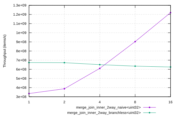
Wow! 😮 When the data is not too skewed (factor 2), the branchless version still performs better. But at factor 4, the naïve version is almost on par with it. And for higher factors, the naïve version wins!

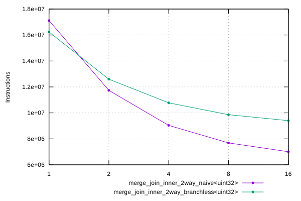
Why? An explanation is that the branchless version simply does more work. It uses more instructions, and in particular more memory writes. When the comparisons are unpredictable, the benefit of avoiding branches is enough to offset the cost of that extra work. But as branches become more predictable, the added cost starts weighing on the performance.

Conclusion🔗

Branchless code can speed up the throughput dramatically if it eliminates unpredictable branches. The more predictable the branches are, however, the less gain is to be expected. In the worst case, the benefits may be completely offset by other costs, for example if the branchless version uses more instructions.